Using the new Turbo palette from Google in R

A couple days ago an AI engineer from Google posted about a new palette he developed. This palette, ‘Turbo’, is as colorful as the widely used ‘jet’ palette, but perceptually uniform and color-blind friendly like the viridis palettes. He shared code in python and C for using the palette, but nothing in R. Others have since posted code in R, though a little work is needed to make it usable with my favorite graphics package, ggplot2. This is a short post on how to quickly get started using Turbo with your ggplots.

EDIT: The code for this post is also now available here: https://github.com/dbaranger/turbo_palette_R

First, we need the actual values for the colors, which are given in sRGB. I then converted these to Hex codes, which is what ggplot2 uses.

install.packages("colorspace")
library(colorspace)

A<-c((0.18995),(0.19483),(0.19956),(0.20415),(0.2086),(0.21291),(0.21708),(0.22111),(0.225),(0.22875),(0.23236),(0.23582),(0.23915),(0.24234),(0.24539),(0.2483),(0.25107),(0.25369),(0.25618),(0.25853),(0.26074),(0.2628),(0.26473),(0.26652),(0.26816),(0.26967),(0.27103),(0.27226),(0.27334),(0.27429),(0.27509),(0.27576),(0.27628),(0.27667),(0.27691),(0.27701),(0.27698),(0.2768),(0.27648),(0.27603),(0.27543),(0.27469),(0.27381),(0.27273),(0.27106),(0.26878),(0.26592),(0.26252),(0.25862),(0.25425),(0.24946),(0.24427),(0.23874),(0.23288),(0.22676),(0.22039),(0.21382),(0.20708),(0.20021),(0.19326),(0.18625),(0.17923),(0.17223),(0.16529),(0.15844),(0.15173),(0.14519),(0.13886),(0.13278),(0.12698),(0.12151),(0.11639),(0.11167),(0.10738),(0.10357),(0.10026),(0.0975),(0.09532),(0.09377),(0.09287),(0.09267),(0.0932),(0.09451),(0.09662),(0.09958),(0.10342),(0.10815),(0.11374),(0.12014),(0.12733),(0.13526),(0.14391),(0.15323),(0.16319),(0.17377),(0.18491),(0.19659),(0.20877),(0.22142),(0.23449),(0.24797),(0.2618),(0.27597),(0.29042),(0.30513),(0.32006),(0.33517),(0.35043),(0.36581),(0.38127),(0.39678),(0.41229),(0.42778),(0.44321),(0.45854),(0.47375),(0.48879),(0.50362),(0.51822),(0.53255),(0.54658),(0.56026),(0.57357),(0.58646),(0.59891),(0.61088),(0.62233),(0.63323),(0.64362),(0.65394),(0.66428),(0.67462),(0.68494),(0.69525),(0.70553),(0.71577),(0.72596),(0.7361),(0.74617),(0.75617),(0.76608),(0.77591),(0.78563),(0.79524),(0.80473),(0.8141),(0.82333),(0.83241),(0.84133),(0.8501),(0.85868),(0.86709),(0.8753),(0.88331),(0.89112),(0.8987),(0.90605),(0.91317),(0.92004),(0.92666),(0.93301),(0.93909),(0.94489),(0.95039),(0.9556),(0.96049),(0.96507),(0.96931),(0.97323),(0.97679),(0.98),(0.98289),(0.98549),(0.98781),(0.98986),(0.99163),(0.99314),(0.99438),(0.99535),(0.99607),(0.99654),(0.99675),(0.99672),(0.99644),(0.99593),(0.99517),(0.99419),(0.99297),(0.99153),(0.98987),(0.98799),(0.9859),(0.9836),(0.98108),(0.97837),(0.97545),(0.97234),(0.96904),(0.96555),(0.96187),(0.95801),(0.95398),(0.94977),(0.94538),(0.94084),(0.93612),(0.93125),(0.92623),(0.92105),(0.91572),(0.91024),(0.90463),(0.89888),(0.89298),(0.88691),(0.88066),(0.87422),(0.8676),(0.86079),(0.8538),(0.84662),(0.83926),(0.83172),(0.82399),(0.81608),(0.80799),(0.79971),(0.79125),(0.7826),(0.77377),(0.76476),(0.75556),(0.74617),(0.73661),(0.72686),(0.71692),(0.7068),(0.6965),(0.68602),(0.67535),(0.66449),(0.65345),(0.64223),(0.63082),(0.61923),(0.60746),(0.5955),(0.58336),(0.57103),(0.55852),(0.54583),(0.53295),(0.51989),(0.50664),(0.49321),(0.4796))
B<-c((0.07176),(0.08339),(0.09498),(0.10652),(0.11802),(0.12947),(0.14087),(0.15223),(0.16354),(0.17481),(0.18603),(0.1972),(0.20833),(0.21941),(0.23044),(0.24143),(0.25237),(0.26327),(0.27412),(0.28492),(0.29568),(0.30639),(0.31706),(0.32768),(0.33825),(0.34878),(0.35926),(0.3697),(0.38008),(0.39043),(0.40072),(0.41097),(0.42118),(0.43134),(0.44145),(0.45152),(0.46153),(0.47151),(0.48144),(0.49132),(0.50115),(0.51094),(0.52069),(0.5304),(0.54015),(0.54995),(0.55979),(0.56967),(0.57958),(0.5895),(0.59943),(0.60937),(0.61931),(0.62923),(0.63913),(0.64901),(0.65886),(0.66866),(0.67842),(0.68812),(0.69775),(0.70732),(0.7168),(0.7262),(0.73551),(0.74472),(0.75381),(0.76279),(0.77165),(0.78037),(0.78896),(0.7974),(0.80569),(0.81381),(0.82177),(0.82955),(0.83714),(0.84455),(0.85175),(0.85875),(0.86554),(0.87211),(0.87844),(0.88454),(0.8904),(0.896),(0.90142),(0.90673),(0.91193),(0.91701),(0.92197),(0.9268),(0.93151),(0.93609),(0.94053),(0.94484),(0.94901),(0.95304),(0.95692),(0.96065),(0.96423),(0.96765),(0.97092),(0.97403),(0.97697),(0.97974),(0.98234),(0.98477),(0.98702),(0.98909),(0.99098),(0.99268),(0.99419),(0.99551),(0.99663),(0.99755),(0.99828),(0.99879),(0.9991),(0.99919),(0.99907),(0.99873),(0.99817),(0.99739),(0.99638),(0.99514),(0.99366),(0.99195),(0.98999),(0.98775),(0.98524),(0.98246),(0.97941),(0.9761),(0.97255),(0.96875),(0.9647),(0.96043),(0.95593),(0.95121),(0.94627),(0.94113),(0.93579),(0.93025),(0.92452),(0.91861),(0.91253),(0.90627),(0.89986),(0.89328),(0.88655),(0.87968),(0.87267),(0.86553),(0.85826),(0.85087),(0.84337),(0.83576),(0.82806),(0.82025),(0.81236),(0.80439),(0.79634),(0.78823),(0.78005),(0.77181),(0.76352),(0.75519),(0.74682),(0.73842),(0.73),(0.7214),(0.7125),(0.7033),(0.69382),(0.68408),(0.67408),(0.66386),(0.65341),(0.64277),(0.63193),(0.62093),(0.60977),(0.59846),(0.58703),(0.57549),(0.56386),(0.55214),(0.54036),(0.52854),(0.51667),(0.50479),(0.49291),(0.48104),(0.4692),(0.4574),(0.44565),(0.43399),(0.42241),(0.41093),(0.39958),(0.38836),(0.37729),(0.36638),(0.35566),(0.34513),(0.33482),(0.32473),(0.31489),(0.3053),(0.29599),(0.28696),(0.27824),(0.26981),(0.26152),(0.25334),(0.24526),(0.2373),(0.22945),(0.2217),(0.21407),(0.20654),(0.19912),(0.19182),(0.18462),(0.17753),(0.17055),(0.16368),(0.15693),(0.15028),(0.14374),(0.13731),(0.13098),(0.12477),(0.11867),(0.11268),(0.1068),(0.10102),(0.09536),(0.0898),(0.08436),(0.07902),(0.0738),(0.06868),(0.06367),(0.05878),(0.05399),(0.04931),(0.04474),(0.04028),(0.03593),(0.03169),(0.02756),(0.02354),(0.01963),(0.01583))
C<-c((0.23217),(0.26149),(0.29024),(0.31844),(0.34607),(0.37314),(0.39964),(0.42558),(0.45096),(0.47578),(0.50004),(0.52373),(0.54686),(0.56942),(0.59142),(0.61286),(0.63374),(0.65406),(0.67381),(0.693),(0.71162),(0.72968),(0.74718),(0.76412),(0.7805),(0.79631),(0.81156),(0.82624),(0.84037),(0.85393),(0.86692),(0.87936),(0.89123),(0.90254),(0.91328),(0.92347),(0.93309),(0.94214),(0.95064),(0.95857),(0.96594),(0.97275),(0.97899),(0.98461),(0.9893),(0.99303),(0.99583),(0.99773),(0.99876),(0.99896),(0.99835),(0.99697),(0.99485),(0.99202),(0.98851),(0.98436),(0.97959),(0.97423),(0.96833),(0.9619),(0.95498),(0.94761),(0.93981),(0.93161),(0.92305),(0.91416),(0.90496),(0.8955),(0.8858),(0.8759),(0.86581),(0.85559),(0.84525),(0.83484),(0.82437),(0.81389),(0.80342),(0.79299),(0.78264),(0.7724),(0.7623),(0.75237),(0.74265),(0.73316),(0.72393),(0.715),(0.70599),(0.69651),(0.6866),(0.67627),(0.66556),(0.65448),(0.64308),(0.63137),(0.61938),(0.60713),(0.59466),(0.58199),(0.56914),(0.55614),(0.54303),(0.52981),(0.51653),(0.50321),(0.48987),(0.47654),(0.46325),(0.45002),(0.43688),(0.42386),(0.41098),(0.39826),(0.38575),(0.37345),(0.3614),(0.34963),(0.33816),(0.32701),(0.31622),(0.30581),(0.29581),(0.28623),(0.27712),(0.26849),(0.26038),(0.2528),(0.24579),(0.23937),(0.23356),(0.22835),(0.2237),(0.2196),(0.21602),(0.21294),(0.21032),(0.20815),(0.2064),(0.20504),(0.20406),(0.20343),(0.20311),(0.2031),(0.20336),(0.20386),(0.20459),(0.20552),(0.20663),(0.20788),(0.20926),(0.21074),(0.2123),(0.21391),(0.21555),(0.21719),(0.2188),(0.22038),(0.22188),(0.22328),(0.22456),(0.2257),(0.22667),(0.22744),(0.228),(0.22831),(0.22836),(0.22811),(0.22754),(0.22663),(0.22536),(0.22369),(0.22161),(0.21918),(0.2165),(0.21358),(0.21043),(0.20706),(0.20348),(0.19971),(0.19577),(0.19165),(0.18738),(0.18297),(0.17842),(0.17376),(0.16899),(0.16412),(0.15918),(0.15417),(0.1491),(0.14398),(0.13883),(0.13367),(0.12849),(0.12332),(0.11817),(0.11305),(0.10797),(0.10294),(0.09798),(0.0931),(0.08831),(0.08362),(0.07905),(0.07461),(0.07031),(0.06616),(0.06218),(0.05837),(0.05475),(0.05134),(0.04814),(0.04516),(0.04243),(0.03993),(0.03753),(0.03521),(0.03297),(0.03082),(0.02875),(0.02677),(0.02487),(0.02305),(0.02131),(0.01966),(0.01809),(0.0166),(0.0152),(0.01387),(0.01264),(0.01148),(0.01041),(0.00942),(0.00851),(0.00769),(0.00695),(0.00629),(0.00571),(0.00522),(0.00481),(0.00449),(0.00424),(0.00408),(0.00401),(0.00401),(0.0041),(0.00427),(0.00453),(0.00486),(0.00529),(0.00579),(0.00638),(0.00705),(0.0078),(0.00863),(0.00955),(0.01055))
  
turbo_colormap_data<-cbind(A,B,C) 
turbo_colormap_data_sRGB<-sRGB(turbo_colormap_data)
turbo_colormap_data_HEX = hex(turbo_colormap_data_sRGB)

Now lets take a look at the palette:

install.packages("pals")
library(pals)

TurboPalette<-colorRampPalette(colors = turbo_colormap_data_HEX ,space="rgb", interpolate = "spline")
pal.test(TurboPalette)

Overall Turbo performs quite well. One area where it’s lacking is the luminosity curve (grey line, bottom-right panel). Luminosity peaks half-way through the palette, so using the entire palette for a continuous scale may not work well in all situations.

Finally, I wrote a shorter helper-function to make it easier to integrate the palette into ggplot2:

Turbo <- function(pal.min = 0,pal.max = 1,out.colors = NULL,pal = turbo_colormap_data_HEX,reverse = F) {
 # pal.min = lower bound of the palette to use [0,1]
 # pal.max = upper bound of the palette [0,1]
 # out.colors = specify the number of colors to return if out.colors = 1, will return pal.min color. if unspecified, will return all the colors in the original palette that fall within the min and max boundaries
 # pal = vector of colors (HEX) in palette
 # reverse = flip palette T/F - performed as last step
  
  if(pal.min == 0){pal.start = 1}
  if(pal.min > 0){pal.start = round(length(pal)*pal.min) }
  pal.end = round(length(pal)*pal.max )
  out = pal[pal.start:pal.end]
  
 if(!is.null(out.colors)){
   pal2 = colorRampPalette(colors = out ,space="rgb", interpolate = "linear")
   out = pal2(out.colors)
 }
  if(reverse == T){out = rev(out)}
  return(out)
}

This function will subset the palette, and will output a specified number of colors if asked (useful for categorical variables).

Now lets take it for a spin! Below I plot on categorical variable, and one continuous variable, in plots borrowed from http://r-statistics.co/.

The categorical variable is a waffle chart. Note below that I’ve commented-out the original coloring, which was a colorBrewer scale, and replaced it with a manual scale with colors supplied by my new Turbo() function:

var <- mpg$class  # the categorical data 
nrows <- 10
df <- expand.grid(y = 1:nrows, x = 1:nrows)
categ_table <- round(table(var) * ((nrows*nrows)/(length(var))))
categ_table
df$category <- factor(rep(names(categ_table), categ_table))  

ggplot(df, aes(x = x, y = y, fill = category)) + 
  geom_tile(color = "black", size = 0.5) +
  scale_x_continuous(expand = c(0, 0)) +
  scale_y_continuous(expand = c(0, 0), trans = 'reverse') +
 ####scale_fill_brewer(palette = "Set3") +####
  scale_fill_manual(values = Turbo(out.colors = 7))+ ## This is the change
  labs(title="Waffle Chart", subtitle="'Class' of vehicles",
       caption="Source: mpg") + 
  theme(panel.border = element_rect(size = 2),
        plot.title = element_text(size = rel(1.2)),
        axis.text = element_blank(),
        axis.title = element_blank(),
        axis.ticks = element_blank(),
        legend.title = element_blank(),
        legend.position = "right")

I’ve replaced: “scale_fill_brewer(palette = “Set3″)” with “scale_fill_manual(values = Turbo(out.colors = 7))”.

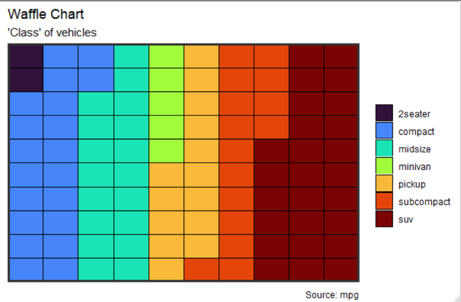
If we don’t like the coloring on that, the ends are pretty dark, we can change the min and max of the palette: “scale_fill_manual(values = Turbo(out.colors = 7,pal.min = .1,pal.max = .9))”

Much better! Now lets try this with a continuous scale, like a heatmap, again borrowed from http://r-statistics.co/.

library(ggplot2)
library(plyr)
library(scales)
library(zoo)
df <- read.csv("https://raw.githubusercontent.com/selva86/datasets/master/yahoo.csv")
df$date <- as.Date(df$date)  # format date
df <- df[df$year >= 2012, ]  # filter red years
# Create Month Week
df$yearmonth <- as.yearmon(df$date)
df$yearmonthf <- factor(df$yearmonth)
df <- ddply(df,.(yearmonthf), transform, monthweek=1+week-min(week))  # compute week number of month
df <- df[, c("year", "yearmonthf", "monthf", "week", "monthweek", "weekdayf", "VIX.Close")]
# Plot
ggplot(df, aes(monthweek, weekdayf, fill = VIX.Close)) + 
  geom_tile(colour = "white") + 
  facet_grid(year~monthf) + 
  ###scale_fill_gradient(low="red", high="green") +##
  scale_fill_gradientn(colours = Turbo()) + ## this is new
  labs(x="Week of Month",
       y="",
       title = "Time-Series Calendar Heatmap", 
       subtitle="Yahoo Closing Price", 
       fill="Close")

Note that I’ve replaced “scale_fill_gradient(low=”red”, high=”green”)” with “scale_fill_gradientn(colours = Turbo()) “.

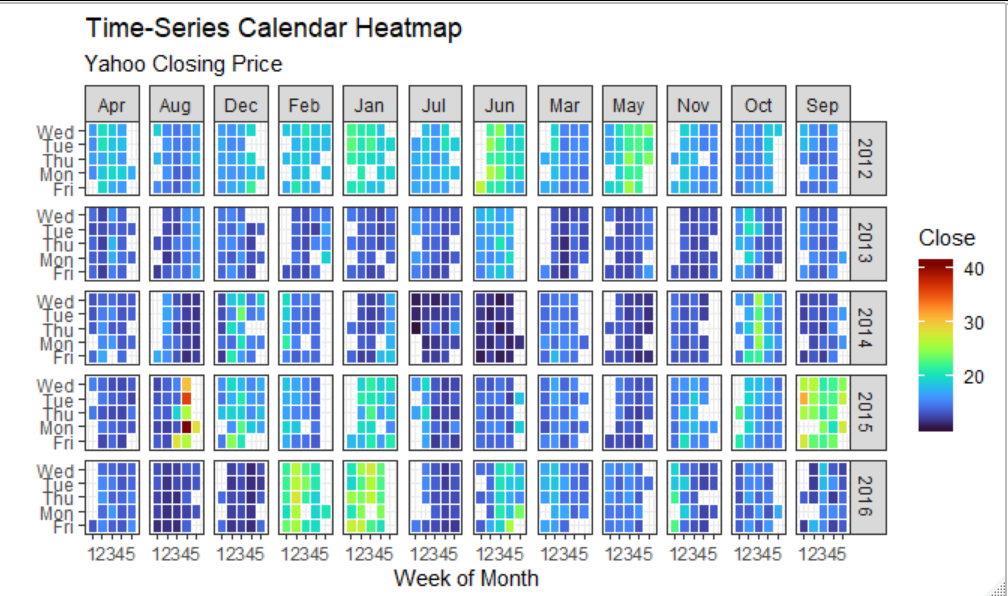
One issue with the above plot is that the green ‘pops’ too much, so we pay attention to middle-values, instead of the maximum. This is because, as the first figure above showed, the luminosity curve peaks half-way through the palette, in the greens. So we can instead plot with a subset of the colors, and flip the palette so that lighter colors are higher. Here I’ve changed the fill to: “scale_fill_gradientn(colours = Turbo(pal.min = .6,pal.max = 1,reverse = T))”

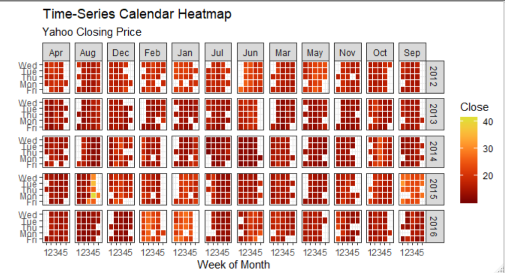
Now it’s much more clear which days contain the highest values.

That’s all for now, happy ggplotting!