

Edit 8/9/22: This ideas discussed in this blog series are now published as a tutorial paper.
Edit 5/24/21: I’ve turned the code underlying these posts into an R package: https://dbaranger.github.io/InteractionPoweR. I’d recommend using this package for your own power analyses, rather than the original posted code, as it’s a lot easier to use, has more features, and I’ve fixed some minor errors.
I conduct interaction (aka ‘moderation’) analyses a lot. As a result, I was interested to read commentaries online about interaction analyses, and the question of how large of a sample is required [1,2]. More recently, results from massive replication efforts, like the Reproducibility Project, have found that interactions were among the effects least likely to replicate [3].
When I first read them, I found these commentaries somewhat difficult to follow, and I thought: “Maybe I don’t understand interactions as well as I thought? Do all interactions need a huge sample size? I thought they were just another variable in my linear model.”
What follows is an attempt to restate these arguments for my past self:
- This post: How to do a power analysis for an interaction in a linear regression (in R), and what factors effect how much power you have.
- Part 2: Interpreting the effect-size of an interaction, by connecting it to simple-slopes.
- Part 3: Determining what sample size is needed for an interaction.
R-code for the analyses, simulations, and figures in this post can be found here.
First, some real data
Using publicly available data from https://openpsychometrics.org/ [4], I tested an interaction. Participants completed several surveys, including Depression, Anxiety, and Perceived Stress, as well as a brief personality survey (Big 5), and some demographic questions. They all agreed to make their responses available for research (no one was paid – the surveys are used more like an online personality questionnaire someone might do online for fun). You can see my steps for filtering and quality control in the R doc for this post, but briefly I’ll say that I’m only using responses from respondents in the United States (or with an IP address in the US), who said they were over 18, who didn’t have missing data, and who didn’t fail a pretty basic validity-check.
Anxiety and neuroticism are strongly associated with perceived stress. I tested whether there was a significant interaction (i.e. an anxiety-by-neuroticism), controlling for various demographic variables including age, sex, sexual orientation, number of siblings, education, ethnicity, and urbanicity. All the variables were standardized (mean is 0 and standard deviation is 1). The sample size is N=1,700, so DF = 1,675.
Call:
lm(formula = Stress ~ age + gender + White + Suburban + College +
    Heterosexual + familysize + Anx + N + Anx:N + (Anx + N):(age +
    gender + White + Suburban + College + Heterosexual + familysize),
    data = DASS4)
                   Estimate Std. Error t value Pr(>|t|)
(Intercept)       0.0373975  0.0169867   2.202  0.02783 *
Anx:N             0.0873982  0.0162109   5.391 7.99e-08 ***
Anx               0.5802001  0.0184820  31.393  < 2e-16 ***
N                -0.3293825  0.0187527 -17.565  < 2e-16 ***
age               0.0485193  0.0156328   3.104  0.00194 **
gender           -0.0101972  0.0152473  -0.669  0.50372
White             0.0004681  0.0149604   0.031  0.97504
Suburban         -0.0268078  0.0148041  -1.811  0.07034 .
College          -0.0115615  0.0153877  -0.751  0.45255
Heterosexual      0.0163745  0.0148892   1.100  0.27160
familysize       -0.0099285  0.0148598  -0.668  0.50413
age:Anx           0.0189089  0.0185720   1.018  0.30876
gender:Anx       -0.0015383  0.0183065  -0.084  0.93304
White:Anx        -0.0249086  0.0173450  -1.436  0.15117
Suburban:Anx     -0.0146885  0.0175529  -0.837  0.40282
College:Anx      -0.0029976  0.0182831  -0.164  0.86979
Heterosexual:Anx -0.0095487  0.0165095  -0.578  0.56309
familysize:Anx   -0.0022462  0.0179375  -0.125  0.90036
age:N             0.0216759  0.0180634   1.200  0.23031
gender:N         -0.0108077  0.0174722  -0.619  0.53629
White:N          -0.0087409  0.0173806  -0.503  0.61509
Suburban:N        0.0276818  0.0173809   1.593  0.11143
College:N         0.0163651  0.0179572   0.911  0.36225
Heterosexual:N   -0.0043325  0.0176113  -0.246  0.80571
familysize:N     -0.0071348  0.0184509  -0.387  0.69903
Signif. codes:  0 ‘***’ 0.001 ‘**’ 0.01 ‘*’ 0.05 ‘.’ 0.1 ‘ ’ 1
So we see a significant interaction of anxiety and neuroticism predicting perceived stress. That is, the correlation between anxiety and perceived stress varies slightly, depending on how neurotic a person is.
I’ll note that the neuroticism scale used in this survey is the reverse of what is more typical, so a lower number means more neurotic. I’ll also note that I’ve included covariate-by-interaction-term interactions in the model (e.g. not only Anxiety x Neuroticism, but also Anxiety x Age, Anxiety x Sex, etc.), to control for possible sources of confounding, per the recommendations of several papers [5,6,7].
A power analysis
Now that we have this result, we might ask, “How large a sample do I need to replicate this?” Or alternatively, “am I powered to detect this effect in the current analysis?”. Both can be answered with a power analysis. If we run a standard power analysis as if this is a simple regression with an independent variable B=0.087 (the effect size of the above interaction), we would get:
pwr.r.test(r = 0.087,power = 0.8,sig.level = 0.05)

     approximate correlation power calculation (arctangh transformation)

              n = 1033.84
              r = 0.087
      sig.level = 0.05
          power = 0.8
    alternative = two.sided
Which would suggest we need approximately N=1,000 to have 80% power to detect this effect. By ‘power‘ I mean that, if we sampled a new set of participants from the same distribution as the original study, with N=1,000 we would see a significant (p<0.05) effect 80% of the time. Clearly, there are good reasons to want more power (you would get a non-significant result 1/5 of the time with 80% power), but it’s a commonly-used standard.
To do a power analysis for my interaction, I used a slightly modified version of the sample code from the ‘paramtest’ R package vignette. The basic idea here is to simulate data with the given effect-size of interest, and to test how frequently you get a significant result with a given sample size. As opposed to a power analysis for a regression, where only one effect-size needs to be specified, here we need four: (1) the interaction term bXM; (2 & 3) main effects of the two interacting variables bX & bM; (4) the correlation (r) between X&M (rXM). All are standardized effect sizes and adjusted for all covariates.
In the present case, bXM = 0.087, bX = 0.58, bM = -0.33, and rXM = 0.5. Again, see the R doc for the full code. Results were as follows:

Our power analysis indicates that with N=1,700 we have great power to detect our effect, and that if we wanted to replicate it, N=500 would give us approximately 80% power. N=500 is half of the N=1,000 we got from out previous analysis, which is something I return to below.
Is this power analysis correct? One way of testing this is to ask how likely we would be to detect a significant effect if we had only analyzed a subset of our actual data. For instance, we would predict that if we chose N=500 of our participants at random, 80% of the time the interaction would be significant. We can actually do this and see if the simulations are correct.
What I did was bootstrap new samples from the original data set. Bootstrapping just means drawing a random sample, with replacement, so that each random sample is different from every other random sample. Then I ran the interaction analysis, and tested how frequently p<0.05 was observed. Again, see the R doc for the full code. Results were as follows:

The results (right-panel) are strikingly similar to our simulations (left-panel), and indicate that N=500 is approximately when we achieve 80% power with this analysis. This tells us that the simulations are doing their job and give us a fairly accurate estimate of our power for an analysis.
Effects of interacting-variable effect size and correlation
Our power analysis says N=500 for 80% power, but the power analysis for a simple regression with the same effect size (B=0.087) says N=1,000. What gives? So I decided run some simulations varying either (A) the correlation between our two interacting variables X and M (rXM) or (B) the effect-size of one of our interacting variables (bX).
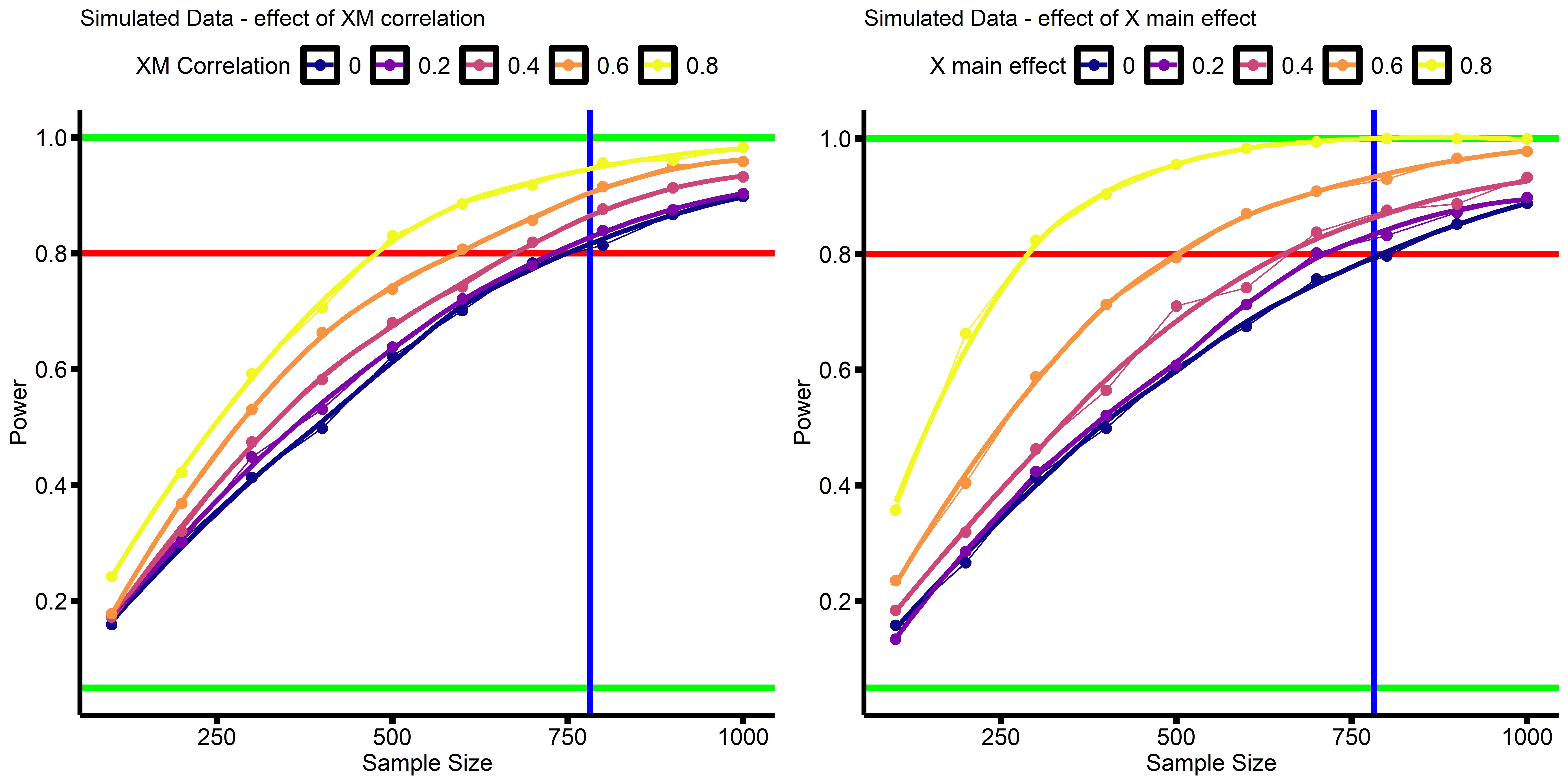
Each dot represents the percent of analyses (1,000 simulations per dot) that found p<0.05 results for the interaction term, at a given sample size. Sample size ranged from N=100-1,000, at increments of N=100. Dots are connected by straight lines, and a smoothed curve was added. Green horizontal lines are at Power = 0.05 and Power = 1.00 (5% and 100% power, respectively). The red horizontal line is at 80% power. The blue vertical line is at N=782, the sample size required to detect a main effect of B=0.1 with 80% power in a regression.
These simulations show that when the main effects, or the correlation between main effects, become medium-to-large, a smaller sample is required to detect the same interaction effect. This is why we only need N=500 in the earlier analyses to detect a the effect of B=0.087, because the main effects of anxiety and neuroticism are large, and the two are highly correlated. However, when the main effects are small, and X & M are not correlated, it is sufficient to run a your power analysis treating the interaction term as a simple main effect of interest (i.e. the horizontal blue lines in the above figure).
That is, if you treat your interaction-term as just a simple linear effect you’re trying to detect, a standard power analysis should give you a conservative idea of how many subjects you need.
Final thoughts and next steps
The results here suggest that, all else being equal, we should be better powered (or at least similarly powered) to detect interactions, relative to similarly-sized main effects. The fact that interactions have a fairly poor track-record suggests that something else is going on.
In doing these simulations I realized that I didn’t have a good sense of the correspondence between an interaction effect size and the actual shape of the data. In part 2 I discuss how the interaction effect size in a regression connects to the simple-slopes of your data. In part 3 I build on this intuition, restating prior commentaries, but in regression terms, that interactions need large sample sizes because we’re interested in small effects. In part 4 I then go on to discuss what covariates are needed when conducting an interaction analysis.
p.s. This post is of course not comprehensive, and ignores other factors that impact power, perhaps most prominently the issue of measurement reliability.

[…] the previous entries to this series I talked about computing power for an interaction analysis (Part 1), interpreting interaction effect-sizes (Part 2), and what sample size is needed for an […]
LikeLike
[…] Part 1 I covered some aspects of what affects power for an interaction analysis, and in Part 2 I talked […]
LikeLike
HI David, thanks for this post! There’s a part of this analysis I didn’t quite understand. You write that you wanted to do a power test to check the necessary sample size for an /effect size/ B=0.87 in a regression analysis, but I see that the following test is a power analysis for correlation (prw.r.test) with a /linear correlation coefficient/ r=0.87. Maybe I’m misunderstanding something? I thought correlation coefficients and effect sizes were very different things? Just to be clear: It looks to me like you’re testing the necessary sample size to detect a correlation of 0.87, not a linear regression effect of 0.87.
LikeLike
Hi! Thanks for the question! The purpose of that part of the post is to get a general idea of what the power would be if the effect were isolated (as opposed to being in the context of a regression with other predictors). Since a standardized regression coefficient (when there is only one IV in the regression) is identical to the Pearson’s correlation, I use the Pearson’s correlation power function. The point is that power for the interaction term is a lot higher than for the effect alone, because the main effects are so large. Does that clarify things?
LikeLike
Love this post and your InteractionPoweR package! Is there currently a way to extend it to estimating a 3-way interaction?
LikeLike
Very glad you like it! Unfortunately, not all the details for 3-way interactions have been worked out yet (to my knowledge). If you assume your variables are independent, you can do a change in R2 power analysis yourself (just sum up the R2s) (the hard part is figuring out how to do the power analysis if variables are correlated).
LikeLike