
Edit 8/9/22: This ideas discussed in this blog series are now published as a tutorial paper.
Edit 5/24/21: I’ve turned the code underlying these posts into an R package: https://dbaranger.github.io/InteractionPoweR. I’d recommend using this package for your own power analyses, rather than the original posted code, as it’s a lot easier to use, has more features, and I’ve fixed some minor errors.
In the previous post in this series I discussed how to compute power for an interaction (moderation) analysis. In writing that post, I realized that I didn’t have a good intuition for the correspondence between standardized effect sizes and the actual shape of the data. Admittedly, I don’t have the greatest sense of what a standard linear effect looks like either (check out http://guessthecorrelation.com/ if you want to see how good you are), but I at least have a general sense.
If a main-effect is bX = 0.3, with an interaction of bXM = 0.1, what does the data look like?
A simple example – binary moderator
First I started with a simple analysis, where the moderator is binary, coded as either 0 or 1, and there are exactly the same number of both values.

The slope of x1=0 is b=0.26, and the slope of x1=1 is b=0.39. The difference in slopes is 0.13, which is exactly the effect-size of the interaction. If we had instead coded our binary moderator as either -1 or 1, the main-effect of x2 would be 1.5 times as large (bX=0.32) and interaction effect would shrink by half (bXM=0.065). The difference of slopes between the two levels of the moderator would stay the same (0.13), which would then be exactly twice the effect-size of the interaction.
Note that this can be generalized for any values of a uniformly distributed binary moderator, where the difference in slopes will be the interaction effect-size multiplied by the difference in the values of the moderator (1-0 = 1, 1 – -1 = 2, etc).
Extending to a continuous moderator
Simple-slopes is common approach to interpreting interaction analyses when the moderator is continuous. In essence, the slope of x on y is examined at different ranges of values of the moderator. Conventionally, three slopes are examined, and their range is defined by the mean and standard deviation of the moderator (usually 1.5xSD). If our moderator has values from 0 to 10, with an average of 5, and a standard deviation of 2, then the groups will be [0 – 2), [2 – 8], (8 – 10].
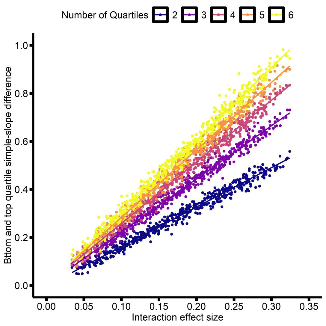
Building on the results with a binary moderator, I thought it would make sense look at ranges defined by the quartiles of the distribution, rather than the standard deviation. That way there will be the same number of observations in each simple-slope. So I simulated several hundred interactions, and examined the relationship between the effect-size and the difference in simple slopes (e.g. if there are 4 groups, then the difference between the 1st and 4th quartiles). I decided to limit this to interaction effect-sizes between 0.05 and 0.3, as that’s the range that strikes me as most plausible for psychological/neuroscience research.

We see that for any effect size, the difference between the simple-slopes of the of the top and bottom quartiles are linearly proportional to the effect size. By ‘top’ and ‘bottom’ I mean, for any number of quartiles, the ‘bottom’ is the first (e.g. quartile #1 if there are 4 quartiles), and the ‘top’ is the last (e.g. quartile #4 if there are 4 quartiles). I extended this to 15 quartiles and 10,000 simulations, and computed the slope of the relationship between the interaction effect size and simple-slope difference, as well as their correlation.
| Quartiles | Slope | Correlation |
| 2 | 1.63 | 0.99 |
| 3 | 2.21 | 1.00 |
| 4 | 2.57 | 1.00 |
| 5 | 2.83 | 1.00 |
| 6 | 3.03 | 1.00 |
| 7 | 3.19 | 1.00 |
| 8 | 3.32 | 1.00 |
| 9 | 3.44 | 0.99 |
| 10 | 3.54 | 0.99 |
| 11 | 3.63 | 0.99 |
| 12 | 3.71 | 0.99 |
| 13 | 3.78 | 0.99 |
| 14 | 3.85 | 0.99 |
| 15 | 3.91 | 0.99 |
The difference in slopes is highly correlated with the interaction effect-size, with the slope of the relationship increasing with more quartiles. If we examine the association between the Slope and the number of Quartiles, we find that there is a strong logarithmic association:
Call:
lm(formula = Slope~ log(Quartiles), data = quart_comparison)
Coefficients:
                 Estimate Std. Error t value Pr(>|t|)
(Intercept)      1.00341    0.05489   18.28 3.97e-10 ***
log(Quartiles)   1.09602    0.02641   41.49 2.49e-14 ***

Multiple R-squared:  0.9931,	Adjusted R-squared:  0.9925
F-statistic:  1722 on 1 and 12 DF,  p-value: 2.488e-14
That is to say, for an interaction effect size bXM, the difference between the simple-slopes of the top and bottom quartiles Q will be approximately: bXM * (ln(Q) +1)
That isn’t intuitive, but I think in most cases you probably only need to think about two or three quartiles to get a general sense for the effect size. For two quartiles the slope difference is just over 1.5-times the interaction effect, and for three quartiles it’s just over 2-times the interaction effect.
Final thoughts and next steps
If we return to my initial question: If a main-effect is bX = 0.3, with an interaction of bXM = 0.1, what does the data look like? We can now say for three quartiles, the difference in slope between the bottom and top quartiles is ~0.1 * 2, or 0.2, So the slope of the bottom quartile is ~0.2, and the slope of the top quartile is ~0.4.
I think this can be useful for interpreting data, and I think it can also be useful planning analyses. In the next post in this series, I’ll show how this little bit of extra intuition can greatly simplify power analyses for interactions. Finally, the fourth post, I go on to discuss which covariates are needed when conducting a test of an interaction.

[…] computing power for an interaction analysis (Part 1), interpreting interaction effect-sizes (Part 2), and what sample size is needed for an interaction (Part 3). Here I’m going to talk […]
LikeLike
[…] Part 2: Interpreting the effect-size of an interaction, by connecting it to simple-slopes. […]
LikeLike
[…] Part 1 I covered some aspects of what affects power for an interaction analysis, and in Part 2 I talked about interpreting interaction effect-sizes in terms of their ‘simple slopes’. […]
LikeLike