
The crowdAI openSNP Height Prediction Challenge
crowdAI is a VERY cool site that hosts machine learning competitions. They recently hosted a competition using data from openSNP, a website that lets anyone upload their genetic data, making it publicly available. About 3,500 people have uploaded some amount of their genetic data (many people just upload the mitochondrial portion), and 921 also reported their height. The crowdAI competition was, very simply, can you predict Height in a subset of these people, using the genetic data from everyone else to train a model?
And? I won!!! My best model predicts 53.45% of variance in Height, while the current next-best predicts 48.62%. But there’s a catch, even though it was a “machine learning”” competition, I didn’t actually use any ML…oops
This post is intended to give an explanation of why I participated and how I won, with the hope that others with more expertise in ML can benefit from my knowledge in genetics.
[EDIT]: If you’re reading this, you may also be interested in the follow-up post, where I further improve this model by an additional 11%.
Why I Participated
I’m a PhD student studying both Neuroscience and Genetics. This is exactly the sort of problem that I spend my days thinking about. For my research it’s often more ‘does genetic-risk for given disorder predict how much people use a certain part of their brain during a psychological task?’, but the underlying techniques are the same. In fact, I recently co-taught a summer workshop on applying behavioral genetics research techniques in psychology and neuroscience. I actually first found the crowdAI competition because I was looking for demo data I could give the workshop participants.
I remembered the competition a month after the workshop ended, and when I came back to it I saw that there were many submissions that were predicting only ~40% of variance in a subset of the final testing dataset (14 people). This struck me as being awfully close to how much variance I would expect a person’s biological sex to predict.
So, I decided to submit my ‘researcher’s best-guess’. NOT because I wanted to put-down machine learning, but because I wanted a benchmark to compare the ML submissions against. I fully expected someone to beat my guess. But, it’s important when doing machine learning to make sure that the baseline model is something reasonable, which is a point this recent paper makes. I then tried to improve on this with some of my own machine-learning, with no luck.
Actually, this whole situation reminds me of the ADHD-200 Competition, which was to correctly classify ADHD patients based on their resting-state fMRI connectivity brain-networks. Turns out, the winner didn’t need to use any of the brain-data whatsoever!
Don’t get me wrong, I’m very interested in Machine Learning. I think it has a lot of potential to aid in the study of human genetics. This paper from Dr. Kristin Nicodemus, where she uses random-forest to identify a non-linear interaction between three mutations that increase risk for schizophrenia, is one of my favorite studies. It was also one of the main inspirations for my NSF Graduate Research Fellowship application (ps. thank you NSF for funding me!), which proposed to combine machine learning with genetics and neuroimaging. Dr. Nicodemus hasn’t given up on machine-learning either – here are the slides to a recent talk she gave on the subject. Also, see this recent paper for an example of machine learning applied to the study of Height. But, if you look at the twitter discussion surrounding it, you’ll note that the fact that they didn’t include the approach I used for this competition is considered a red flag.
I think this experience also has some lessons for organizers of ML competitions, more generally. Using just my knowledge of genetics, I was able to generate a model that was simply a description of the dataset – sex + 3 principal components – which performed as well as the average machine learning submission. These are the sort of things that organizers might provide to the contestants, especially if expert-knowledge in an area isn’t supposed to be a prerequisite.
Moving Forward
Part of my motivation for posting this is that I would like to give the other participants in the competition (and anyone else who’s interested) the chance to surpass this “baseline”. You can find a file with the five variables in my final regression – yes, literally only 5 variables in a simple linear-regression beat who knows how many neural-nets – HERE.
The Analysis – Outline
The model I built that ended up winning had 5 main steps to it:
- Setup data for analysis
- Guess people’s biological sex (it wasn’t provided)
Sex can be very predictive of Height. It’s in the genes (Y&X Chromosome), but the data from the competition didn’t include it. Luckily, it’s quite easy to impute.
- Remove related people from the training data
Generally, for a genetic analysis, you want the degree of relatedness across participants to be relatively constant. This is frequently simply that everyone is equally un-related. Alternatively, you might have families, where there are a subgroups of people who are vastly more-related to each other than they are to anyone else. In the case of the training data for this competition, neither was the case. The participants are generally totally unrelated, with a small handful of people who are direct relatives. This can be a problem, because it will bias your model towards being good only at predicting the height of people in those families, instead of predicting the height of anyone.
- Generate Principal Components
The openSNP data is multi-ethnic. That is, the majority of the participants are white, but there’s also a good number of people of African and Asian descent. This is a problem, because it virtually guarantees increased false-positives. Principal components analysis is the standard baseline way to 1) identify that your sample is multi-ethnic (in genetics we call this ’population stratification), and 2) generate an initial, but not complete or entirely sufficient, correction.
- Create a Polygenic Risk Score (PRS) for Height
Polygenic risk scores are worthy of a post all by themselves. They are the standard technique researchers in behavioral genetics apply when trying to predict a trait in an independent sample. Polygenic risk scores (PRS) are not a new approach. I’m not entirely sure which was the first paper to use them, but certainly by the early 2000’s. They’re extremely simple, so it’s pretty remarkable that they have proven to be so useful. A PRS starts with an independent study, a GWAS, where every allele in the genome is independently tested to see whether it predicts a trait. The PRS is then constructed by taking a new sample, and for each participant in that sample adding-up all the risk-alleles they have, weighted by the effect-size of the allele in the first sample. For a PRS you most-often include only the SNPs that are below a certain p-value threshold in the discovery sample. You might think that a fairly stringent threshold, say only those SNPs whose p-value survives bonferroni-correction for multiple tests, would work best. One of the more surprising observations from PRS analyses is that typically a very lenient threshold, say p<0.5 uncorrected, or even p<1.0 (aka every single SNP), works best.
In schizophrenia, the PRS-approach can now capture upwards of 20% of disease-risk. Here’s a GWAS published this July that used a PRS in a validation sample. The main caveat with the PRS approach (and honestly with all human genetics research) is that it works best when everything is done within the same ethnic sample. Multi-ethnic samples, or samples of entirely different ethnicities than what was used in the discovery GWAS, will see worse/poor performance.
In this competition, each team was provided with a curated set of ~900 alleles that are known to be associated with Height. These alleles were identified in a 2014 GWAS of Height. The crowdAI organizers did the hard job of variable-selection for each team beforehand. Now, the results of this GWAS are publicly available here. I simply downloaded them and used them to generate a PRS for Height.
[EDIT]: While not exactly the same, the PRS-approach might be thought of as an extremely simplified version of ensemble learning. Given N SNPs, we fit N experts, where each expert is a regression trained on a single feature. We then compute a weighted average of the experts, where the weight-vector is the effect-size of the feature in each regression. While this approach virtually guarantees that we won’t capture the maximum amount of variance possible, it also seems to be very good at reducing overfitting. I think this is an especially important point for genetics research, where each individual feature has a very small effect-size. More complex learning-algorithms thus run the risk of latching onto effects which appear to be especially predictive, but are actually just noise.
The Analysis in Detail
A note on software
I mostly ran my analyses in plink and R. Almost all the code below is R-code – even the plink-code is written as a system call through R. R is my software-of-choice (one day soon I will probably encounter a problem that I actually need to know python for, but that hasn’t happened yet), and calling plink through R is convenient, because it makes scripting and loops very easy. Also, I’m writing this with RMarkdown 🙂
1) Setup data for analysis
The first step is to convert the g-zipped .vcf files provided by crowdAI to the plink binary format. anything problematic.
system(paste ("plink --vcf genotyping_data_fullset_test.vcf --biallelic-only strict --make-bed --out OpenSNP_test",sep=" "))
system(paste ("plink --vcf genotyping_data_fullset_train.vcf --biallelic-only strict --make-bed --out OpenSNP_train",sep=" "))
VCF files can be a pain, with lots of variables named “.” and other errors. For the purposes of the competition I decided to ignore them all and just throw-out anything problematic.
library(data.table)
Train_bim<-fread(c("OpenSNP_train.bim"))
Train_bim2<-filter(Train_bim, V2 != ".")
Train_bim4<-Train_bim2[!duplicated(Train_bim2[c('V2') ]),  ]

write.table(x=Train_bim4$V2,file=c("SNPS_keep.txt"),sep="",quote = F,col.names = F,row.names = F)
rm(Train_bim, Train_bim4, Train_bim2)

system(paste ("plink --bfile OpenSNP_train --extract SNPS_keep.txt --make-bed --out OpenSNP_train2",sep=" "))
system(paste ("plink --bfile OpenSNP_test --extract SNPS_keep.txt --make-bed --out OpenSNP_test2",sep=" "))
Now we merge them, and throw-out anything else problematic (right, not the best practice for research, but it works for the purposes of the competition)
system(paste ("plink --bfile OpenSNP_train2 --bmerge OpenSNP_test2 --make-bed --out OpenSNP_combined",sep=" "))

system(paste ("plink --bfile OpenSNP_train2 --exclude OpenSNP_combined-merge.missnp --make-bed --out OpenSNP_train3",sep=" "))
system(paste ("plink --bfile OpenSNP_test2 --exclude OpenSNP_combined-merge.missnp --make-bed --out OpenSNP_test3",sep=" "))

system(paste ("plink --bfile OpenSNP_train3 --bmerge OpenSNP_test3 --make-bed --out OpenSNP_combined2",sep=" "))
Finally, catch the rest of the errors, and remove them too (NB this isn’t a lot of SNPs)
Errors<-readLines(c("OpenSNP_combined2.log"))
Rem<-as.data.frame(matrix(NA,length(Errors),1))
for (i in 1: length(Errors)){
  Mult<-regexpr('Warning: Multiple positions seen for variant',Errors[i])
       if(Mult>0){Rem[i,1]<-substr(Errors[i],47,(nchar(Errors[i])-2)) }
  Dup<-regexpr('Warning: Variants ',Errors[i])
       if(Dup>0){
                 And<-regexpr(pattern = 'and',Errors[i])
                 Rem[i,1]<-substr(Errors[i],20,(And[1]-3))
                  }
}

Rem<-na.omit(Rem)

write.table(x=Rem$V1,file=c("SNPS_remove.txt"),sep="",quote = F,col.names = F,row.names = F)
system(paste ("plink --bfile OpenSNP_combined2 --exclude SNPS_remove.txt --make-bed --out OpenSNP_combined3",sep=" "))
2) Guess Biological Sex
Now that we have everyone in one plink file, with no errors, we can guess their biological sex. This is done with the plink –impute-sex flag, which computes X-chromosome inbreeding coefficients. First we need to prune-out correlated snps (see the plink documentation).
system(paste ("plink --bfile OpenSNP_combined3 --indep-pairphase 20000 2000 0.5 --make-bed --out OpenSNP_combined4",sep=" "))
system(paste ("plink --bfile OpenSNP_combined3 --extract OpenSNP_combined4.prune.in --make-bed --out OpenSNP_combined5",sep=" "))
system(paste ("plink --bfile OpenSNP_combined5 --impute-sex ycount --make-bed --out OpenSNP_combined6",sep=" "))
Let’s take a look at that file
library(data.table)
Sexcheck<-fread("OpenSNP_combined6.sexcheck")
hist(Sexcheck$F)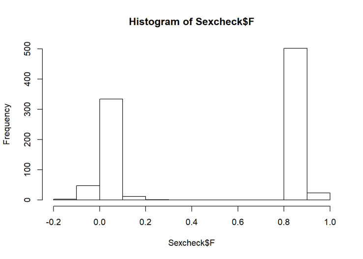
table(Sexcheck$SNPSEX)##
## 0 1 2
## 1 524 396We see a nice separation of F-scores, indicating that it’s probably pretty accurate. However, there is one person the algorithm isn’t certain about. They’re probably biologically female (F=0.2), but I’m going to remove them anyway. Then we can make the first model!
library(dplyr, quietly = T,warn.conflicts = F,verbose = F)

Height<-fread('phenotypes.txt') #This is the training data Heights
Sex2<-merge(Sexcheck,Height, by="IID")
Sex2<-filter(Sex2, SNPSEX > 0)
fit1<-lm(Height ~ SNPSEX, data = Sex2)
summary(fit1)
##
## Call:
## lm(formula = Height ~ SNPSEX, data = Sex2)
##
## Residuals:
## Min 1Q Median 3Q Max
## -26.4193 -5.0445 -0.0445 5.5807 23.5807
##
## Coefficients:
## Estimate Std. Error t value Pr(>|t|)
## (Intercept) 193.7941 0.8433 229.8 <2e-16 ***
## SNPSEX -14.3748 0.5571 -25.8 <2e-16 ***
## ---
## Signif. codes: 0 '***' 0.001 '**' 0.01 '*' 0.05 '.' 0.1 ' ' 1
##
## Residual standard error: 7.719 on 781 degrees of freedom
## Multiple R-squared: 0.4602, Adjusted R-squared: 0.4595
## F-statistic: 665.7 on 1 and 781 DF, p-value: < 2.2e-16Unsurprisingly, biological sex is a good predictor of Height, capturing ~46% of variance – women are shorter than men. Now, we generate predictions.
Sex3<-as.data.frame(setdiff(Sexcheck$IID,Sex2$IID))
colnames(Sex3)<-c("IID")
Sex3<-merge(Sex3,Sexcheck, by = "IID")
Sex3<-filter(Sex3, SNPSEX > 0)
Sex3$pred2<-predict(fit1,Sex3)
write.table(Sex3$pred2,file="PredSex2.txt",sep = ",",col.names = F,row.names = F)
Here’s how this prediction – that each person’s height is the average for their sex, stacks-up. In the independent test set, sex alone predicts 42.08% of the variance.

3) Remove Related People
So, the next step will be to identify family members, and remove them. I used plink’s –genome flag, which computes an estimate of identity by descent. IBD reflects how related two people are:
1.00 = Same person or monozygotic twins
0.50 = Parent/child or siblings
0.25 = First cousins
etc…
A cutoff of 0.1875 (halfway between 1st and 2nd cousins) is pretty typical.
So I’ll pull out all the IBDs above a low threshold, 0.05, and plot everything above IBD=0.1.
system(paste ("plink --bfile OpenSNP_combined5 --genome --min 0.05 --out OpenSNP_combined5_IBD",sep=" "))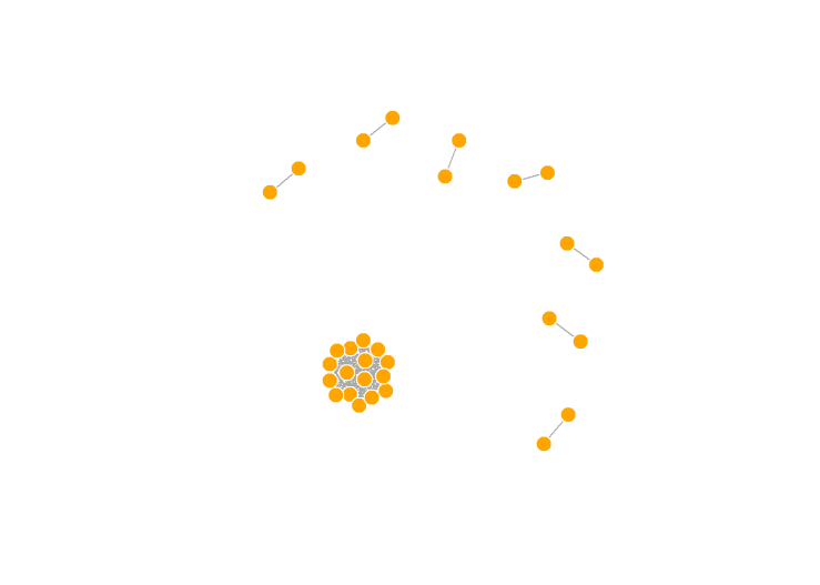
We see several pairs of participants that are strongly related, and then one HUGE clump of people who are all related to each other. In reality, these people are all 3rd cousins, but that extended family is waaaayy larger than one would expect by chance. Keep in mind, these are all people who voluntarily uploaded their genotype data to a public website and made it totally open. People do this for many reasons, though one would be if they have a disease of some sort that runs in the family, they may hope to learn more about it.
I removed one member from each pair with an IBD > 0.1875, and all but one of the people in the huge clump.
Train_Exclude<-c(567, 191, 849, 796, 569, 680, 461, 706, 688, 457, 746, 737, 263, 390, 61, 529, 55, 338, 492, 846, 392, 511, 901, 457)
Train_Exclude<-cbind(Train_Exclude,Train_Exclude)
write.table(x=Train_Exclude, file="TrainExclude.txt", sep=" ", quote = F, row.names = F, col.names = F)
system(paste ("plink --bfile OpenSNP_combined3 --remove Train_exclude.txt --make-bed --out OpenSNP_combined7",sep=" "))
4) Generate Principal Components
We can use plink to generate the top 20 principal components
system(paste ("plink --bfile OpenSNP_combined7 --pca 20 --out PCs20_SNP7",sep=" "))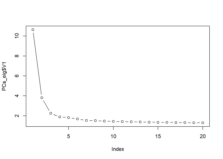
We see that the first PC has a very large eigenvalue. This is a hallmark of population stratification.
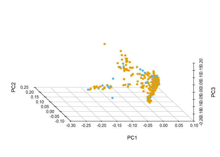
Orange is training and blue is test. This is the canonical shape of a multi-ethnic sample(see Figure 5 here). That clump near the origin is where all the White people are, while the tails are African and Asian descent (NB it’s the canonical-shape of a mostly-white sample).
Since both training and test samples are multi-ethnic, I didn’t remove anyone in this step. In retrospect, maybe I should have. If I removed all the non-white people from the training data, that would probably improve my prediction in the majority of the test sample, which would improve my over-all model performance.
But, for my actual submission, I just corrected for the top-three principal components. For research, this would probably not be sufficient. Here’s what that looks like:
Sexcheck<-fread("OpenSNP_combined6.sexcheck")
Sex2<-merge(Sexcheck,Height, by="IID")
Height<-fread('phenotypes.txt')

Sex2<-merge(Sexcheck,Height, by="IID")
Dat<-merge(PCs, Sexcheck, by = "IID")
Test<-fread('OpenSNP_test.fam')
colnames(Test)[1]<-"IID"
Test<-merge(Test,Dat, by="IID")

Train<-merge(Height, Dat, by="IID")

Fit_all<-lm(as.formula(paste("Height ~ SNPSEX + ", paste("PC",c(1:3),sep="",collapse = "+") )),data=Train)
summary(Fit_all)
##
## Call:
## lm(formula = as.formula(paste("Height ~ SNPSEX + ", paste("PC",
## c(1:3), sep = "", collapse = "+"))), data = Train)
##
## Residuals:
## Min 1Q Median 3Q Max
## -25.4227 -5.2219 -0.1535 5.0593 22.3754
##
## Coefficients:
## Estimate Std. Error t value Pr(>|t|)
## (Intercept) 193.9242 0.8474 228.838 < 2e-16 ***
## SNPSEX -14.4399 0.5630 -25.648 < 2e-16 ***
## PC1 20.3413 9.0280 2.253 0.024537 *
## PC2 -28.0329 8.3567 -3.355 0.000835 ***
## PC3 18.6254 8.1439 2.287 0.022470 *
## ---
## Signif. codes: 0 '***' 0.001 '**' 0.01 '*' 0.05 '.' 0.1 ' ' 1
##
## Residual standard error: 7.651 on 756 degrees of freedom
## Multiple R-squared: 0.4672, Adjusted R-squared: 0.4644
## F-statistic: 165.7 on 4 and 756 DF, p-value: < 2.2e-16The principal components improve our model performance in the training data by ~0.5%

Similarly, the principal components improve the performance in the testing data by ~1%. Now the model explains 43.28%.
5) Create a Polygenic Risk Score
Dr. Sarah Medland has an excellent presentation online on how to create polygenic risk scores. I’m not going to go into all the details. I use PRSice to create my PRS. Well actually, I use a custom R-script based on PRSice, because PRSice is linux-only and doesn’t easily produce results at the thresholds I want, but the result is the same. I generated PRS for Height at several different thresholds, I plot the amount of additional variance they explain in the training sample, below.

We see that the PRS explains an additional 6.9% – 10.0% of the variance, with the threshold p<0.00001 performing best. While this would be amazing performance for almost any other trait (genetics analyses are still only able to predict a small fraction of the variance of a trait, in most cases), this is honestly pretty poor for Height (physical traits are easier to predict than more complex things, like IQ, and Height has been very thoroughly studied). The poor performance is likely due to the multi-ethnic sample.
Here’s how that model compares in the test set:

The PRS explains an additional 10% of variance in the test-data. It’s nice to see that it performs roughly as well in the test as in the training data!
So that’s how I did it. No machine-learning, just expert-knowledge. As I said above, I’m sharing these results in hopes that others might be able to improve on them. If you do, please give me a shout!!

Thanks for this! This is a great example of how expert knowledge of how to process your features will blow naive machine learning out of the water every time.
LikeLike
nicely done, but I would like to see one additional thing: how does this procedure perform on a randomized phenotype ? This would give you an estimate of the amount of overfitting in your procedure.
LikeLike
Thanks for the feedback., though, if I understand you correctly, I think the performance in the independent test-data (N=137) already addresses your question. In the training-data the model explained ~54.5% of the variance, while in the test-data it explains 53.4%, indicating minimal over-fitting.
If your question is with regard to the polygenic score itself, I don’t think overfitting is a concern as 1) the weights are taken from a large independent study (N=250,000), 2) I don’t re-estimate the weights before computing the score (https://www.ncbi.nlm.nih.gov/pmc/articles/PMC4096801/), and 3) polygenic risk score results are more replicable than anything else we’ve seen in human genetics (other than family-based heritability).
LikeLike